Motivation

The problem with using a normal band-pass filter for EEG analysis is that the output is an oscillating signal, and you'd have to do peak-detection to find the amplitude. Given the short duration of transient features in the EEG stream, it would be much better to have a continuous (DC) signal as output from the filter.

For example, we have this wavelet in the input data that we want to detect, corresponding to about 5 wavelengths at 12Hz in 256Hz sampled data:

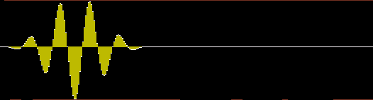
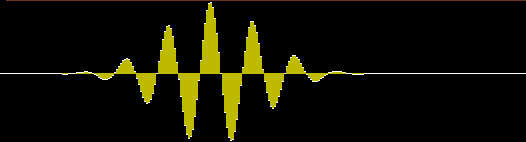
Passing it through a band-pass filter (centered on 12Hz with 4Hz width at -3dB), we get the following signal as output, which is not adequate for our purposes:

Overview of technique

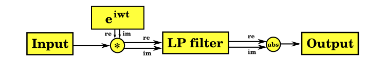
The input signal is multipled by the output of a complex oscillator (e^iwt) and the result of the multiplication is passed through a low-pass filter before the modulus (absolute value) of the complex number is taken. The oscillator runs at the centre frequency of the band to be detected (F), and the low-pass filter width (0 to W Hz) should be half the required width of the band (since the low pass filter really operates from -W to W Hz, which when frequency-shifted corresponds to F-W to F+W Hz). This gives a continuous (DC) output.

Applying this technique to the example wavelet above, with the same filter width and centre frequency, we now get this output:

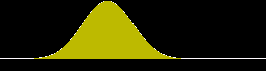
A nice smooth output like this, which reflects the amplitude envelope of the input wavelet rather than its oscillations, is much easier to use in further processing.

Theory

Take an example input sine wave:

    2*A*cos(a*t)

which can also be written:

    A * (e^iat+e^-iat)

Apply the complex oscillator:

    A * e^iwt * (e^iat + e^-iat)

giving:

    A * (e^i(w+a)t + e^i(w-a)t)

Apply the low-pass filter F(w):

    A * (F(w+a) * e^i(w+a)t + F(w-a) * e^i(w-a)t)

Assuming the low-pass filter is efficient and appropriate to the frequencies being tested [*], then F(w+a) will be close to 0, so we can drop that term, giving:

    A * F(w-a) * e^i(w-a)t

Taking the modulus gives:

    A * F(w-a)

So, we have successfully extracted the amplitude of the sine wave (A) as a continuous value with no oscillations to worry about.

This assumes perfect unchanging infinite-length waves, as do most filter analysis proofs!! In real life A is a function of time A(t), and this amplitude envelope interacts with the envelope of the low-pass filter by convolution. So as a rule of thumb, the length of the measured amplitude envelope will be roughly the length of the input amplitude envelope plus the length of the filter envelope (i.e. the length of the filter impulse response).

[* Note: for this technique to work properly the low-pass filter must give F(w+a) close to zero for all positive 'a'. So for a centre frequency of 15Hz, the low-pass filter must give near zero response at 15Hz and above. If the F(w+a) term isn't near 0, then that term remains and this introduces an oscillating interference to the output magnitude. A practical filter's response never quite goes to zero, so you need to bear in mind that there will be a small oscillating error in your output magnitude corresponding to whatever small amount of signal is leaked through your filter. Check the response of your filter at and above the centre frequency to see whether it is acceptable for your application, and if it isn't, then narrow your filter width or select a higher order filter (which also has its trade-offs).]

Applying the technique with IIR filters

The stages can be executed exactly as described above. For example, here is some example code adapted from EEGMIR, which uses IIR filters generated with fidlib:

      // 'input' is current input sample
      // 'lp0' and 'lp1' are working buffers for low-pass filters
      // 'osc' is a working buffer for generating the complex oscillator
      // 'output' is output of filter
      double val = input;
      sincos_step(osc);
      double re = lp_func(lp0, val * osc[0]);
      double im = lp_func(lp1, val * osc[1]);
      double output = hypot(re, im);

The sincos_step() function steps the complex oscillator forward one angular increment corresponding to the sample period. Of course you could just evaluate sin(w*t) and cos(w*t) functions but it is more efficient to do it as a complex multiplication with a constant value (e^ia), as is done in EEGMIR. The low-pass filter lp_func() must be applied separately to the real and imaginary parts of the signal after multiplication by the complex oscillator -- i.e. there are really two low pass filters running here side by side. The amplitude (modulus) is taken using the hypot() function which does (re²+im²)^0.5 internally.

Compared to a simple IIR band-pass filter, twice the calculations are required (two filters) plus the oscillator and hypot() calculations (two multiplies and a square root).

The low-pass filter should be selected bearing in mind the normal trade-off of sharpness in frequency response against sharpness in time response, i.e. a very sharp frequency cut-off gives very poor time-response, so transient features would go undetected. For best recognition of transient features, simple Bessel IIR filters give a nice quick and localised time-response, as well as a good locality of frequency response, although the response is domed rather than square.

Applying the technique with FIR filters

Rather than executing the stages as described above, it is possible to pre-multiply the complex oscillator into the FIR filter. This means that the phase is fixed instead of changing, but as we are extracting the modulus, we don't care about the phase (and anyway we could compensate for the fixed phase if that was necessary). So we take the FIR, and pre-multiply it by the complex oscillator output resulting in two FIR filters, one giving the real part of the result, and the other giving the imaginary part. The modulus of this complex output value can be taken as before to give the result.

As with IIR, the low-pass FIR filter should be selected to give good transient detection. Window functions are well suited to this. (Window functions are all low-pass filters). Using a Blackman window, for example, the code to set up the FIR filters could be as follows (to make the example simple, parameters are hardcoded):

      // Length of filter, which determines impulse response length
      // and filter width (in frequency).
      #define LEN 109

      // Number of waves within filter, which determines center
      // frequency.
      #define WAVES 5
      
      double filt[LEN], filt_re[LEN], filt_im[LEN];
      
      void
      setup() {
         // Basic Blackman window; see fidlib source for more flexible
         // parameterised Blackman creation code
         int wid = (LEN+1)/2;
         memset(filt, 0, sizeof(filt));
         for (int a = 0; a<wid; a++) {
            filt[wid-a] = filt[wid+a] = 0.42 +
                  0.5 * cos(M_PI * a / wid) +
                  0.08 * cos(M_PI * 2.0 * a / wid);
         }
      
         // Multiply with complex oscillator
         for (int a = 0; a<LEN; a++) {
            double theta = 2 * M_PI * WAVES * a / LEN;
            filt_re[a] = filt[a] * sin(theta);
            filt_im[a] = filt[a] * cos(theta);
         }
      }

The code to apply it might look like this:

      double
      calculate(double *input) {
         double tot_re = 0, tot_im = 0;
         for (int a = 0; a<LEN; a++) {
            tot_re += filt_re[a] * input[a];
            tot_im += filt_im[a] * input[a];
         }
         return hypot(tot_re, tot_im);
      }

Compared to using an FIR band-pass filter, twice the calculations are required (two FIR filters), plus the square root in the hypot(). However, there is an additional optimisation possible when using FIR filters with this technique. Because the output of the filter calculation is continuous (DC) rather than fluctuating (AC), it is not necessary to calculate every output sample in order to do peak-detection. So it is possible to sample the output at a lower frequency, and still be sure to detect all the features. For example for EEG data at 256Hz, perhaps the FIR filters could be applied once every 8 or 16 samples, resulting in output at 32Hz or 16Hz. This means that using this technique, the filters require much less CPU power than a band-pass FIR.

For fast integer FIR calculations (e.g. in a DSP chip), the only tricky part of this method is calculating the square root in integers. There are some code samples here. You need to allow 16 iterations to calculate the square root of a 32-bit number. However, if a squared signal value is acceptable for later calculations, then the square root can be skipped, e.g. using re*re+im*im directly instead of calculating (re²+im²)^0.5.

These pages and files, including applets and artwork, are Copyright (c) 1997-2019 Jim Peters unless otherwise stated. Please contact me if you'd like to use anything not explicitly released, or if you have something interesting to discuss.